Want to control MLS payroll? Get rid of the DP.

The source of all of MLS's financial pressures.

In an earlier post I showed how MLS payroll disparity is not increasing, but that the average team payroll did increase by nearly $750,000 from 2005 to 2009. Now I will go through and explore the sources of that increase.

First, I will state the obvious: one source of this increase is likely due to the designated player (DP) rule. But with such a general increase in pay over the five year period, perhaps there has been a natural growth in everyone's salaries over those years. We know that the salary cap has increased each year, and the MLS has a pretty liberal interpretation of the salary cap. Thus, I will test whether the DP, the passing of seasons of play, or both are to contribute to the increase in team payroll.

To do this, I am going to build a General Linear Model (GLM). The GLM is a more general case of a Design of Experiments model, but it has the benefit of not requiring a balanced data set. One doesn't have to have the same number of each combination of variable settings, just one combination of each at a minimum - this is important as the number of teams with DP's fluctuates from season-to-season. A GLM tests multiple variables with multiple settings all at the same time. This is a better test method than one-factor-at-a-time (OFAT) testing, as it allows one to observe any interactions in the variable set (i.e. passing years and increasing DP salaries combining to raise team payrolls). In this case, the two factors of interest are each passing season of play and whether or not a team has a DP, with the response variable being team payroll. This allows the GLM to look at the means and standard deviations of team payroll for each individual variable as well as the combination of them. We will then be able to tell which individual variables and combinations of variables are significant predictors of team payroll, and which are not.

One of the key changes from my previous analysis is that I will only be able to analyze 2007 through 2009 data. This is because the GLM does require at least one combination of the variables for each data set. Thus, if I included 2006 I would not be able to have two sets of team payrolls (with DP, without DP) because the DP did not exist in 2006. This would violate the rules of GLM and my statistical software package would not be able to compute the GLM's statistics.

In this case, it is best to think of the variables and their settings in this GLM as a 3 x 2 matrix. Each team's payroll has been assigned an appropriate year value and a team status value. In the case of the year, I simply renumbered 2007 as "1", 2008 as "2", and 2009 as "3". Thus, the 3x2 matrix of factors looks like:

• Year: 1, 2, 3
• Team Status: DP, no DP

You can see the original data set here.

One of the first steps in the GLM analysis is to normalize the response variable of team payroll, which we know from the previous post is not normal once DP's were introduced. To do this, I first divided each payroll by a million to make the numbers more manageable. I then performed a Box-Cox transform test. The Box-Cox equation is of the form below, and the test is identifying the value of Lambda that shows the best chance of producing a normal data set after the transformation takes place.

y=x^lambda

Figure 1: Box-Cox transform equation and study of team payroll

In this case, I used the rounded value of -2.00. This means that all data is transformed as:

y = (team payroll/1000000)^-2

This transform of the payroll data does indeed produce a normally distributed data set. I then constructed the GLM, using the transformed payroll as the response and the factors identified above. In the first study, I constructed a model that included the interaction between DP and Year Number. Before diving into the results, we must check that the assumptions of the GLM are met.

I will go into the detailed assumptions in a future post on regression, so for right now I will cover their general guidelines. In general. any regression or model should not have a predictable behavior between its predicted response and the actual measured response. In this case, the predicted response is what the GLM predicts the behavior of the transformed payroll data is versus the passing years and whether or not a DP is on the team, while the actual measured response is the actual transformed payroll data. The difference between each predicted response and the corresponding measured response is called a residual. These residuals must be normally distributed, show no discernible pattern versus the predicted value (fits), and shouldn't have a discernible pattern versus the order of the data. The final two conditions protect against some type of bias in the test sample - either in outliers or in the order in which it was gathered. In completing a GLM study, one can have a statistical package compute quantities like residuals and then test them to ensure the pre-requisites for the GLM are satisfied.

Figure 2 shows a four-in-one chart of the residuals from the GLM with interactions between season and DP included. The two plots on the left are a graphical representation of the distribution of the residuals. The data does look like it might be normal, but a specific test will be performed shortly to confirm this. The two plots on the upper right confirm that while there is some spread between predicted values and their residuals, the GLM seems to be okay. The graph on the bottom right confirms random behavior of the residuals based upon the order of the data.

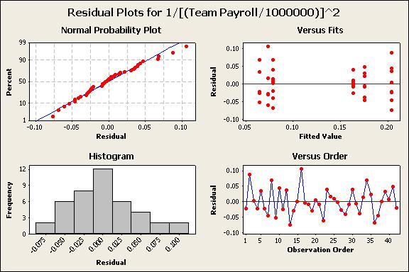
Figure 2: Four-in-One Chart of GLM with interactions

Now it is time to check the normality of the residuals. Figure 3 shows the results of an Anderson-Darling normality test. The p-value of 0.619 indicates that we must accept the null hypothesis that the data is normally distributed. We have now satisfied the basic assumptions of the GLM, and can now move on to analysis of its results.

Figure 3: Graphical Summary of the residuals from the GLM with interactions.

The results of the GLM analysis are in Figure 4. Just like previous statistical tests, the GLM provides p-values to assess the significance of a test - in this case, whether or not that factor is a significant contributor to the prediction of the response variable. P-values that are greater than 0.05 indicate that the factor is likely not significant, and thus can be removed from the analysis. Further analyses can be performed to drill down to the truly significant factors, but all of this must be done one factor at a time. Statements about the relationship between the response variable and predictors can only be made once one has drilled down to only the significant factors.

Figure 4: GLM of payroll, year number, and their interaction

In the case of the GLM with interactions, we see two potentially insignificant factors - year_number and year_number*DP (the interaction effect) - with p-values greater than 0.05 (see far right column of report). Statistical convention requires that one eliminate the most complex term first, and then work down to the less complex factors. In this case, the interaction effect of the year number and DP will be dropped and the GLM will be run again excluding the interaction effect.

The GLM was run again, this time without the interaction effect included. The requirements for residuals were satisfied again, and the results from the GLM are presented in Figure 5.

Figure 5: Results of GLM without interaction effects.

Removing the interaction effects did indeed change the results of the statistical tests. The p-value for year_number has dropped from 0.660 to 0.434, but this is still not below the 0.05 threshold. Meanwhile, the factor representing whether or not a DP is on the team has a p-value of 0.00. The general conclusion from the GLM is that year_number is not a statistically significant predictor of team payroll, but whether or not a team has a DP is a significant predictor.

Now that the GLM has reduced to one factor with two levels, it is no longer useful to use a GLM to analyze the data. It has been reduced to two sample populations, and the difference between them can be tested via a two-sample test. Given that we know the original data is non-normal, and the fact that we are interested in the differences between team payrolls, the non-parametric Mann-Whitney test will be used to quantify the gap between team payrolls with and without DP's. The results of the test are in Figure 6.

Figure 6: Results from Mann-Whitney test of with/without DP

The results of the test show that there is a statistically significant difference in the payrolls of teams with a DP versus teams without a DP, and the gap is just over $1.5M.

General Conclusions

In general, we can conclude that the increase in team payroll over the last CBA was:

• Not due to increases in overall payrolls, but
• Driven primarily by teams who chose to sign a designated player and who spend an average of $1.5M more than teams who don't have a DP.

These conclusions seem odd given the rhetoric surrounding the recent round of CBA negotiations. Team owners seemed very concerned about the financial pressures on their teams, and sought to limit the the growth of every player's salary by fighting free agency proposals, amongst others, from the players union. However, as soon after the new CBA was signed the league came out with changes to the DP rules which would allow teams to purchase a second and third DP if they so choose. Given that only a few teams are profitable and a number of them have chosen to use the DP rule, it seems as if the owners may be speaking out both sides of their mouths. Perhaps they should be looking to modify or eliminate the designated player rule before they look to limit every player's salary.


With all of this focus on payroll and the costs of DP's, the next logical question is:

• Can we equate MLS payroll and/or DP's with some measure of success - table finish, making the playoffs, championships - like Soccernomics did with the top two English football leagues?

I will tackle that topic in a post at a later date. In the meantime, I plan to indulge one of my readers in their request for more details on regression theory by recreating the seminal Soccernomics pay-to-win analysis.

Wherever you're at, I hope you have a great weekend and enjoy some soccer!